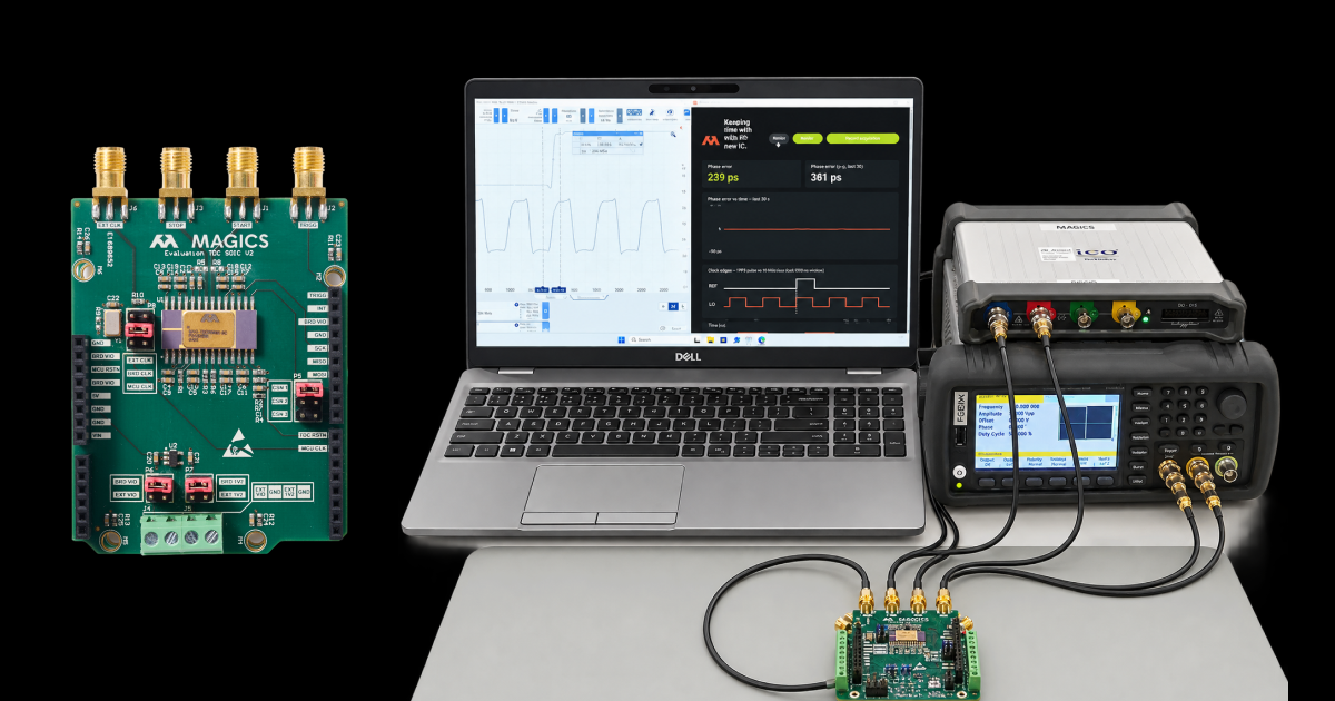
A disciplined oscillator is one of the quiet workhorses of a space payload. It keeps a local clock aligned to a one-pulse-per-second (1PPS) reference, and keeps it running when that reference disappears. Conventionally it is a small analog subsystem: a phase comparator, a DAC, a voltage-controlled crystal oscillator, and the careful design work needed to keep a tuning voltage clean through a mission dose of radiation.
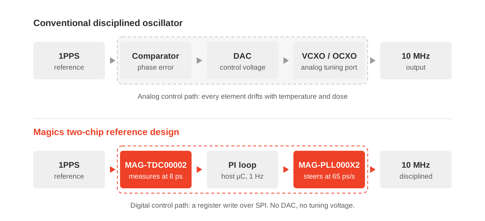
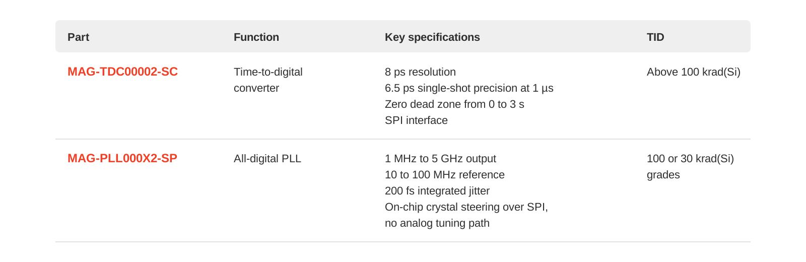
This article describes a Magics reference design that replaces that subsystem with two radiation-tolerant chips, one SPI bus and about a hundred lines of control loop. The MAG-TDC00002 time-to-digital converter measures the timing error at 8 ps resolution. The MAG-PLL000X2 all-digital PLL steers its own crystal over SPI at an effective 65 ps per second. There is no DAC, no tuning voltage and no analog control path anywhere in the loop.
All results below were measured on the bench against a laboratory 1 Hz pulse generator. We have not yet run this loop against a live GNSS receiver, and none of the figures should be read as an end-to-end GNSS-disciplined oscillator result.
The problem every timing chain has to solve
Any timing chain that must ride through a GNSS outage starts with two imperfect clocks:
- The local oscillator is cheap, always available, and wrong. A bare crystal sits tens of parts per million from nominal, which adds up to microseconds of error for every second it runs.
- The 1PPS reference is accurate, but it arrives only once a second and lands on a coarse grid.
Something has to measure the difference between them and steer the oscillator onto the reference. It has to do so tightly enough that the residual error does not matter to the payload, and keep doing it as the radiation dose accumulates.
In a conventional disciplined oscillator, that something is analog. A phase comparator produces the error, a DAC turns the loop's decision into a voltage, and that voltage pulls a VCXO or OCXO through its tuning port. Every element in that path drifts with temperature and dose, and the control voltage must stay clean enough not to become the dominant noise source. Each one has to be designed, qualified and characterised on its own.
The signal chain
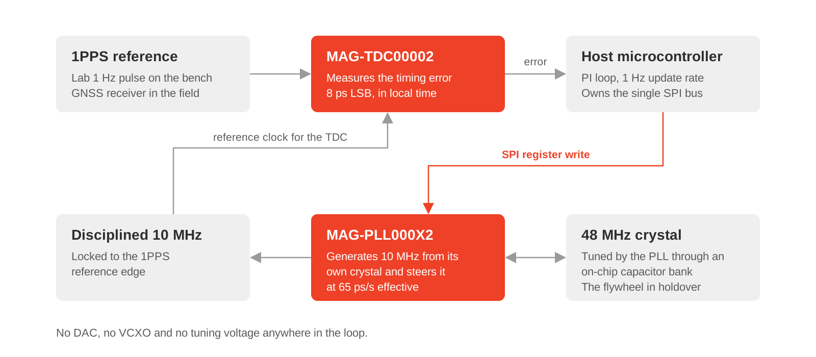
The reference design has three parts: a converter that measures, a PLL that steers, and a small control loop in between.
Measurement: MAG-TDC00002. The time-to-digital converter acts as the phase detector. Its reference clock is the disciplined 10 MHz output itself, so every measurement comes back in units of local time, which is exactly what a disciplining loop needs. Each measurement reads the interval from a trigger aligned to the local clock to the next reference edge.
Steering: MAG-PLL000X2. This is where the design departs from a conventional disciplined oscillator. The all-digital PLL generates the 10 MHz output from its own 48 MHz crystal, and tunes that crystal through an on-chip capacitor bank controlled over SPI. A frequency correction is a register write. By dithering the capacitor bank between adjacent codes, the loop reaches an effective steering resolution of 65 ps of accumulated time per second.
Control: a PI loop on a host microcontroller. A proportional-integral loop runs once per second. The microcontroller owns the single SPI bus and reads the converter only on its completion interrupt.
How the loop acquires lock
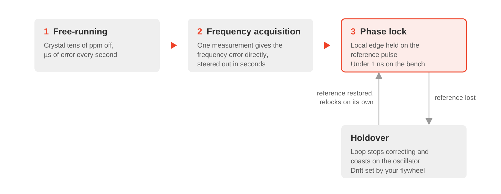
The local clock starts out badly wrong, and the loop brings it in two stages.
Frequency first. Because the converter measures an interval rather than just a polarity, the first pair of pulses already gives the frequency error directly. The loop does not have to watch the phase slide for tens of seconds to infer how fast the oscillator runs. It reads the error and steers it out in seconds. A counter-based front end must trade acquisition time against resolution at this point; a picosecond-class interval measurement does not.
Phase second. With the frequency error nulled, the loop switches to phase control, pulls the local edge onto the reference pulse and holds it there.
Holdover and recovery. Remove the reference and the loop stops correcting, coasting on the oscillator. Restore it and the loop reacquires on its own, without intervention.
What we measured
In a 33-minute continuous cold run against a 1 Hz laboratory pulse generator, the loop held phase lock with zero dropouts and zero outlier rejections. The highlights:
- Alignment stayed inside 1 ns for the whole run.
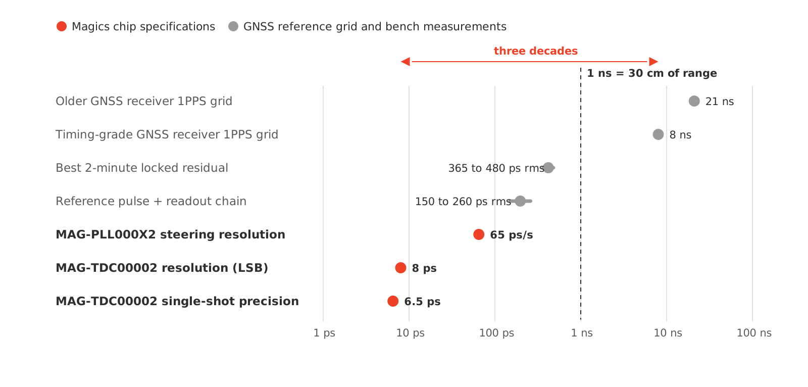
- The best two-minute windows measured 365 to 480 ps rms.
- The crystal's drift rate fell from roughly 16 ppb/s to a little over 0.1 ppb/s as it warmed up, and the loop applied nearly 900 ppb of total correction to follow it.
- Once thermally settled, the frequency residual stayed within ±1 ppb.
The remaining error breaks down as follows, in rank order:
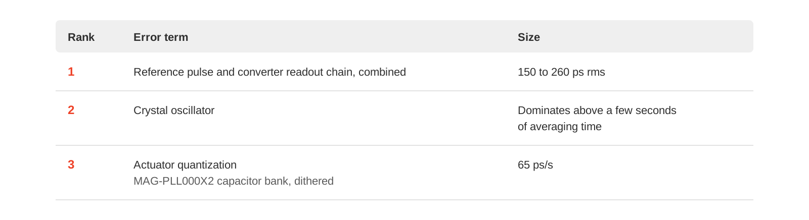
In no configuration we have tested is a Magics chip the limiting term. The electronics have left the error budget; what remains is the oscillator and the reference.
Why picoseconds matter when the reference is quantized in nanoseconds
A GNSS receiver places its 1PPS on an internal clock grid: 8 ns on a current timing-grade receiver, and around 21 ns on older generations that derive the pulse from a 48 MHz clock. A reference quantized at nanoseconds looks like an argument against measuring at picoseconds.
The quantization is knowable, though. Timing receivers report the residual between the pulse they emitted and the pulse they intended, and that residual can be corrected out, but only as well as you can measure it. A front end that resolves the reference to 8 ps and steers at 65 ps/s sits three decades below the grid. The limit of that correction then lies somewhere other than in your own electronics.
Sub-nanosecond timing matters well beyond the clock itself:
- Ranging and geolocation. One nanosecond of timing error is 30 cm of range. Inter-satellite ranging, TDOA emitter location and multistatic radar inherit it directly.
- Distributed coherence. Formation flying, coherent apertures and inter-satellite links need node clocks aligned to a fraction of a carrier period.
- Picosecond-native instruments. Time-of-flight mass spectrometry and single-photon lidar already work in the converter's units.
What this gives you that a catalog part does not
Commercial synchronizer and GPSDO silicon is good, and on raw phase-detector resolution some of it is excellent. The differences that matter for a space timing chain lie elsewhere.
Picosecond resolution through a mission dose. The MAG-TDC00002 is specified above 100 krad(Si) total ionizing dose, and the MAG-PLL000X2 is available in 100 and 30 krad(Si) grades. Today, you cannot assemble a disciplining front end from catalog synchronizer parts and keep picosecond-class measurement resolution through a mission dose.
No analog control path to qualify. There is no DAC, no tuning voltage and no op-amp around a VCXO. Nothing in the control path has a drift or radiation response that you need to characterise separately.
Single-shot specifications that fit a 1PPS reference. A 1PPS reference gives you one edge per second, so there is nothing to average. What governs performance is the converter's 6.5 ps single-shot precision at 1 µs and its zero dead zone from 0 to 3 s. Those are why frequency acquisition takes one measurement instead of a minute.
European supply, no ITAR. Both parts are designed and supplied from Belgium, with no ITAR restrictions.
On holdover: bring your own flywheel
Holdover is half of any timing requirement, and this loop does not set it. When the reference disappears, error accumulates at a rate set by the oscillator you chose as the flywheel.
Our reference design holds over on a plain crystal. That is the worst case by design: it shows the loop working without a premium oscillator propping it up. Fit an OCXO or a chip-scale atomic clock and the holdover figure improves by decades, with no change to the measurement and steering chain described here.
The division of labour is simple. You choose the flywheel your mission needs; the MAG-TDC00002 and MAG-PLL000X2 measure it and steer it, in silicon that survives the environment.
The parts on the board
From analog subsystem to register write
Clock disciplining has long been an analog problem solved with analog parts, each with its own drift, its own radiation response and its own qualification effort. This reference design shows that the whole control path can move into the digital domain. A picosecond-class time-to-digital converter measures the error, an all-digital PLL steers its crystal with a register write, and a hundred lines of firmware close the loop.
On the bench, the result holds a crystal-based 10 MHz clock to a 1PPS reference with sub-nanosecond alignment and best-case residuals below 500 ps rms. The remaining error belongs to the oscillator and the reference, not to the electronics. For missions that depend on ranging, distributed coherence or picosecond-native instruments, that is the point: the timing chain stops being the limit.
This is a reference design rather than a product. If you are building a timing chain for a radiation environment and want to discuss where it fits, contact us.